Model Cascades for Computer Vision: Building a Two-Stage Vision Pipeline
 Timothy MPublished Oct 1, 2026
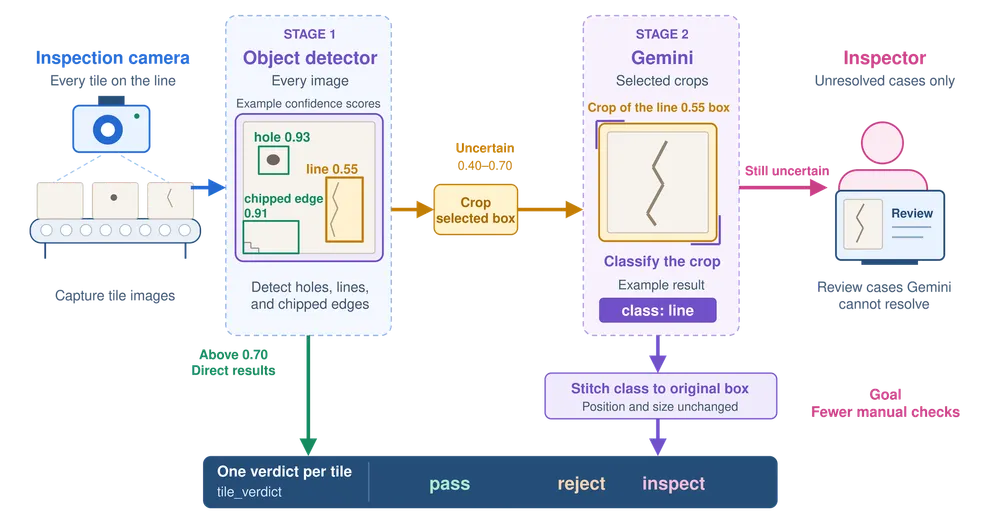
To reduce manual inspection without losing accuracy, build a two-stage model cascade in Roboflow Workflows. RF-DETR runs on every tile and accepts detections at and above 0.70 confidence, while the uncertain ones between 0.40 and 0.70 are cropped and sent to Gemini, and anything Gemini marks “unsure” goes to an inspector in Roboflow Annotate.
Model cascades for computer vision connect models in stages, using an earlier model’s output to guide what a later model analyzes. In a conditional cascade, a fast model handles the initial pass, while selected images or regions receive additional processing. This gives teams a way to balance prediction quality, inference cost, and latency.
With Roboflow Workflows, you can build a cascade that connects object detection, conditional routing, and a second model in one pipeline. For example, a manufacturer inspecting ceramic tiles can use RF-DETR to identify potential defects, send uncertain regions to Gemini for verification, and route unresolved cases to an inspector.
This guide explains how vision model cascades work, when to use them, and how to choose routing rules and second-stage inputs. You’ll build a tile inspection cascade in Roboflow, then learn how to evaluate its accuracy, escalation rate, latency, and cost against your existing inspection process.
What Is a Model Cascade in Computer Vision?
A model cascade in computer vision connects models in sequence, using an earlier model’s predictions to guide what a later model processes. A cascade can combine classifiers, object detectors, segmentation models, or vision-language models, with each stage performing a defined task.
In a conditional cascade, a routing rule determines which images or regions need another model. This lets the system handle straightforward cases with an initial model and apply additional processing where needed. The second model may specialize in a narrower task rather than being more capable across every task.
Common examples include:
- Classifier to classifier: A small model classifies straightforward images and sends uncertain cases to a larger classifier.
- Detector to specialist model: An object detector locates a component, then a specialized segmentation model examines that region to outline a defect.
- Detector to vision-language model: A detector selects relevant images or crops, then a VLM interprets their contents or returns a structured assessment.
Research has explored cascades across image classification, video classification, and semantic segmentation, demonstrating their use beyond detector-to-LLM pipelines.
In this guide, we build two model stages with a human-review fallback using Roboflow Workflows. RF-DETR detects potential tile defects, and a confidence-based routing rule sends selected regions to Gemini for verification. Unresolved cases go to an inspector.
The inspector provides a final review path within the inspection process. The two model stages remain RF-DETR and Gemini, each with its own inputs, outputs, and evaluation criteria.
Why Cascades Work in Practice
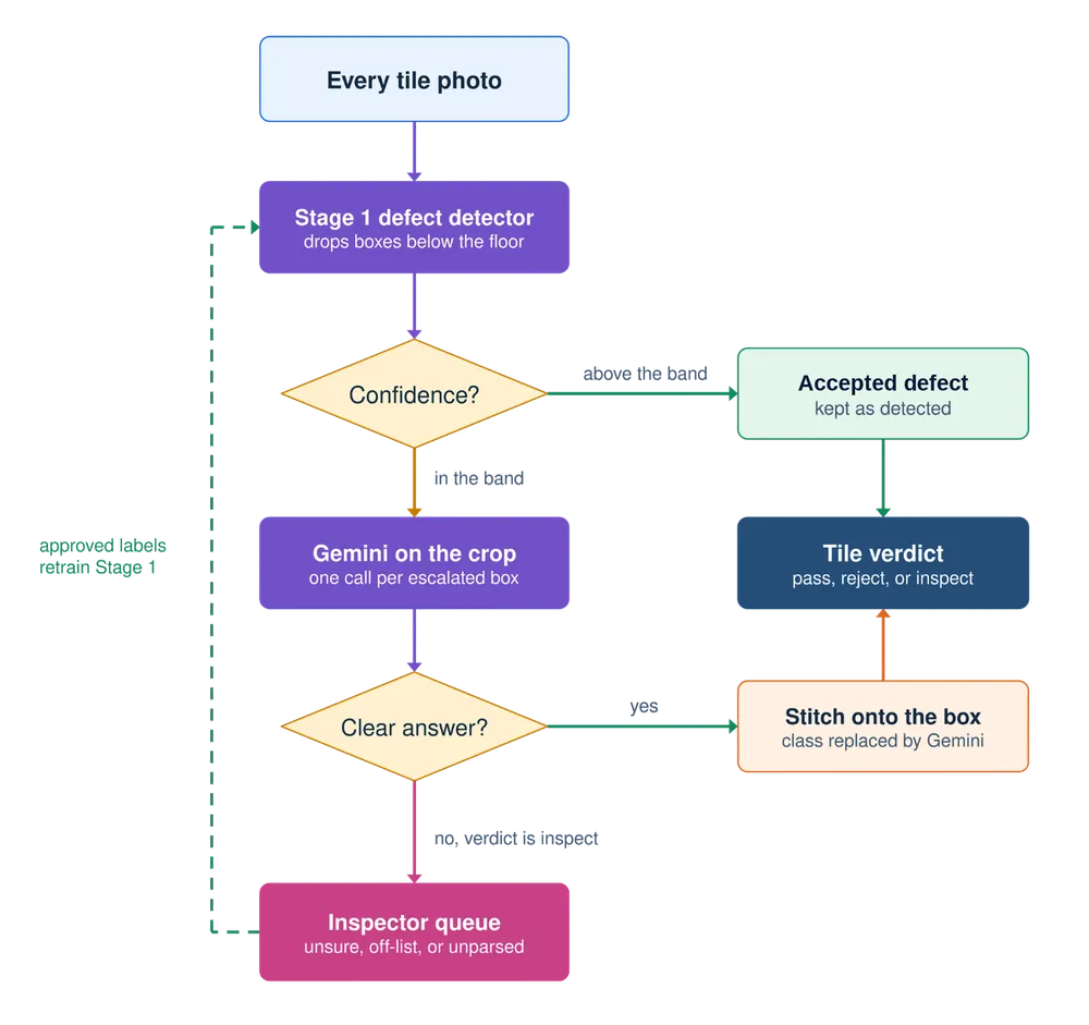
A two-stage design can reduce costs and support better decisions. It follows how quality teams already work. Clear cases are decided quickly, while difficult cases get a closer look. These building blocks also appear in following examples that are worth checking out.
- Surface defect severity assessment sorts parts into PASS, REVIEW, and FAIL. Borderline parts go to a person for review. Severity needs a separate rule because a confident detection does not always mean a serious defect.
- Automated defect rejection uses confidence thresholds, per-defect-class severity, minimum defect size, and frame debounce to make pass and fail decisions. These rules turn the model output into a reject signal and help prevent a single noisy frame from rejecting a good part.
- A VLM production system needs to handle malformed or incomplete model responses in JSON before importing labels. The tile cascade applies the same validation to every Gemini response before using its decision.
Research also supports the use of cascades and deferral.
- Wisdom of Committees (ICLR 2022) studies committee-based models, including ensembles and cascades. Its experiments show that an EfficientNet cascade can achieve a 5.4x speedup over B7 while maintaining the same accuracy.
- Consistent Estimators for Learning to Defer to an Expert (ICML 2020) studies predictors that can make a prediction or defer the decision to a downstream expert. In the tile cascade, Gemini is the first expert, and the inspector is the final expert.
Two design choices remain. They are what Stage 2 receives and where to set the escalation band. The next sections explain each choice in that order.
Three Ways to Send Images to the Second Model
Deciding when to escalate is only half of a cascade. The other half is the input that Stage 2 receives. That input sets how many Gemini/LLM calls you pay for. It also sets what Gemini can actually see.
Shape 1. Filter
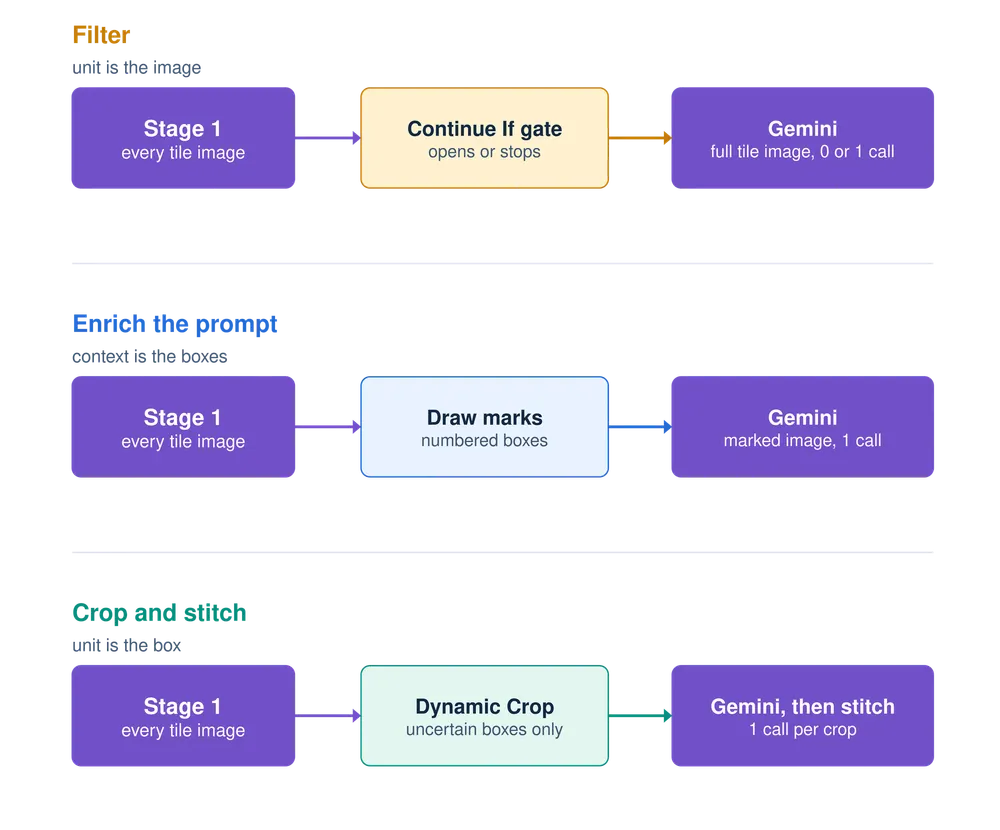
In a filter cascade, Stage 1 decides whether Gemini needs to process an image. If Stage 1 detects an uncertain defect, the entire tile image is sent to Gemini. Otherwise, Gemini is skipped. In Roboflow Workflows, the Continue If block controls this decision based on the detection confidence. This approach saves processing costs when defects are rare. However, Gemini cannot identify defects that Stage 1 completely misses, because those images never reach Stage 2.
Shape 2. Enrich the Prompt
In this approach, Gemini receives the full tile image along with the detections from Stage 1. Bounding boxes, numbers, class names, and confidence scores are drawn on the image to help Gemini identify and review each defect. This method is based on Set-of-Mark Prompting, which uses visual marks to direct a multimodal model's attention to specific image regions.
In Roboflow Workflows, the Bounding Box Visualization and Label Visualization blocks add these marks. This is useful because the Gemini block uses a shared prompt across a batch, while the image marks provide details specific to each tile. Gemini then uses Structured Output Generation to review each numbered box and identify any visible defects that Stage 1 missed. The JSON Parser extracts the results into structured fields.
The main benefit is that Gemini makes only one call per tile, regardless of the number of detected defects. It can also find missed defects because it sees the complete image. However, the drawn labels and boxes may sometimes cover small defects.
Shape 3. Crop and Stitch
In this approach, Stage 1 sends only uncertain defect regions to Gemini instead of the complete tile image. The crop step extracts each uncertain bounding box as a separate image for Gemini to analyze. The stitch step assigns Gemini's classification result back to the corresponding original bounding box, replacing its class label and confidence while keeping its position and size unchanged. Stitching does not mean combining cropped images into one image. It means mapping Gemini's classification results back to the original detections.
This approach helps Gemini focus on small defects without processing unnecessary image areas. Research such as MLLMs Know Where to Look shows that the size of the visual subject can significantly affect multimodal model performance. In Roboflow Workflows, three blocks handle this process:
- Dynamic Crop extracts an image crop for each uncertain detection.
- VLM as Classifier converts Gemini's response into a class label.
- Detections Classes Replacement assigns the predicted class and classification confidence back to the original bounding box.
Gemini is called once per uncertain box. For example, a tile with three uncertain detections requires three Gemini calls, while a tile with none requires no calls. This approach reduces unnecessary image processing and works well for small defects. However, Gemini cannot detect defects that Stage 1 missed because it only receives the cropped regions.
Choosing a Shape
Each shape balances the number of Gemini calls with how much of the tile Gemini can inspect. The table compares the three shapes for a tile inspection line.
| Shape | What Gemini receives | Gemini calls per tile | Catches Stage 1 misses | Best fit |
|---|---|---|---|---|
| Filter | The full tile photo, only when the gate opens | 0 or 1 | Only on tiles where the gate opens | Rare defects in a large stream |
| Enrich the prompt | One tile photo with numbered Stage 1 marks | 1 | Yes | Full-tile audits and missed-defect checks |
| Crop and stitch | One crop per uncertain box | One per uncertain box | No | Small defects and close calls such as hole versus dust |
A production line can combine these shapes. For example, it can run the crop and stitch workflow on every tile, calling Gemini only for uncertain boxes. It can also send a small sample of tiles through enrich the prompt to audit Stage 1 and check for missed defects. The build section uses crop and stitch to give Gemini a closer view of small tile defects.
Escalation Thresholds, Latency, and Cost per Stage
A model cascade needs clear rules to decide when Stage 1 can handle a defect and when Gemini or a human inspector is needed. These rules also affect processing time and cost.
Set the Escalation Thresholds
Stage 1 uses two confidence thresholds to decide what happens to each detection:
- Below 0.40: Ignore the detection because confidence is too low.
- 0.40 to 0.70: Send the uncertain detection to Gemini for further analysis.
- 0.70 or higher: Accept the Stage 1 prediction without escalation.
These values are only starting points. Use your model's Precision, Recall, and F1 scores on validation data to select suitable thresholds. Confidence scores are not always reliable probabilities. A score of 0.70 does not necessarily mean a 70% chance of a correct prediction. Research on model calibration highlights this problem. Different defects may also need different thresholds. For example, faint lines may require a wider escalation range than clearly visible holes. The Detections Filter can filter detections using both class and confidence.
Treat Gemini's Answer as a Label
Gemini's confidence should not be used directly to make escalation decisions because LLMs can be overconfident. Instead, use Gemini's predicted class to decide the next step:
- Valid defect or no-defect label: Use the result according to the inspection rules.
- Unsure , invalid, missing, or unrecognized label: Send the image to a human inspector.
Including an "unsure" option in Gemini's prompt allows it to flag blurry, unclear, or difficult defects rather than forcing a prediction. This approach lets Stage 1 handle clear detections, Gemini examine uncertain cases, and human inspectors review results that remain unresolved.
Budget Latency per Stage
Latency matters because the inspection result must reach the PLC before the tile reaches the reject gate. Each stage adds processing time. Stage 1 adds detector inference time, while Stage 2 adds the Gemini request time.
Cloud LLM calls can add around a second or more per call, so measure it on your line. In an automated defect rejection system, writing the reject bit to the PLC can take tens of milliseconds. A cloud LLM request can therefore take much longer than the PLC write. For two stages running sequentially, estimate the mean latency per tile as:
- T̄ is the mean latency per tile.
- T₁ is the Stage 1 latency.
- q is the share of tiles with at least one escalated box.
- T₂ is the Stage 2 latency for one escalated tile.
The complete timing budget also needs to include image capture, cropping, result processing, and PLC communication. Gemini starts after Stage 1 selects uncertain detections. If a tile has several uncertain bounding boxes, Stage 2 has several image crops to analyze. The Gemini block provides two settings that can help reduce latency:
max_concurrent_requestsallows requests for multiple image crops to run concurrently. Setting it to8permits up to eight requests at once.thinking_levelcontrols reasoning depth for Gemini 3 and newer models. Setting it tolowcan reduce latency and cost for simple inspection tasks.
Mean latency alone does not show whether every tile meets the reject deadline. Even if only 5% of tiles require Gemini, those escalated tiles still need their results in time. Measure their processing times separately.
Pass enable_profiling=True to run_workflow(...) in the Inference SDK to request a profiler trace. When the server enables trace exposure, the trace lets you inspect execution time for each Workflow block. If Gemini cannot return a result within the available time, route uncertain tiles to a hold lane and complete their inspection when the result arrives.
Count Cost per Stage
Cost follows the same split as latency. Stage 1 runs on every tile. Gemini runs once per escalated box. The inspector reviews only what Gemini cannot settle. The mean cost per tile follows the formula below.
- C̄ is the mean cost per tile.
- C₁ is the Stage 1 cost per tile.
- m̄ is the mean number of escalated boxes per tile.
- C₂ is the cost of one Gemini call.
- h is the share of tiles sent to the inspector.
- C_H is the cost of one inspector review.
The table lists the unit latency and cost of each stage.
| Stage | Runs on | Latency | Cost |
|---|---|---|---|
| Stage 1, RF-DETR Small | Every tile | 3.5 ms model time on a T4 | 0.1875 credits per 1,000 images |
| Escalation logic | Every tile | CPU work with no model call | Not billed per image |
| Stage 2, Gemini 3 Flash Preview | Each escalated box | Hundreds of milliseconds per call | Up to 0.28 credits per 1,000 calls for image tokens |
| Stage 2, Gemini 3.1 Pro Preview | Each escalated box | Hundreds of milliseconds per call | Up to 1.12 credits per 1,000 calls for image tokens |
| Inspector review | Tiles that Gemini cannot settle | Set by the review queue | 0.1 credits per 1,000 uploads plus inspector time |
The Gemini rows count image tokens. Each Gemini 3 image uses at most 1,120 tokens at the default media resolution. Prompt text and output tokens add to the image cost. Measure q, m̄, and h on real production tiles. Those three numbers decide whether the cascade pays off.
Build the Tile Inspection Cascade in Roboflow Workflows
In this section, we build a Tile Inspection Model Cascade workflow for ceramic tile inspection using Roboflow Workflows.
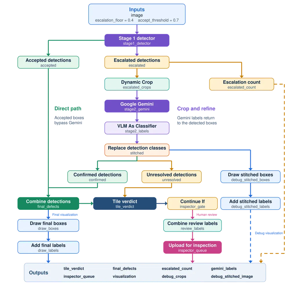
Stage 1 detects possible defects, while Gemini examines uncertain detections. The workflow produces one final verdict for each tile: pass, reject, or inspect.
Step 1. Train Stage 1 and Set the Escalation Band
Start with the trained tile defect model and create a new Workflow in Roboflow. The workflow accepts a tile image and two confidence thresholds:
escalation_floor = 0.40is the minimum confidence needed to consider a detection.accept_threshold = 0.70is the confidence required to accept a detection without Gemini.
Add an Object Detection Model block using the trained RF-DETR Small model. Set confidence_mode to custom and custom_confidence to escalation_floor. This ensures the model returns low-confidence detections that may need further review. Use the class_filter to keep only hole, line, and edge-chipping. Next, add two Detections Filter blocks to divide the predictions:
- Accepted: Detections with confidence greater than or equal to 0.70. These are accepted directly.
- Escalated: Detections with confidence from 0.40 to below 0.70. These are sent to Gemini.
Detections below 0.40 are ignored. This allows Stage 1 to handle clear defects while sending uncertain ones to Stage 2.
Step 2. Ask Gemini About Each Escalated Box
Add a Dynamic Crop block to extract a separate image crop for each escalated bounding box. Connect the crops to the Google Gemini block. Select the Open Prompt task and use the prompt to define the tile defect classes. Gemini can return one of five classes:
hole: A pinhole or pit in the tile glaze.line: A crack or line defect on the surface.edge-chipping: A damaged or broken tile edge.no_defect: Normal texture, glaze patterns, dust, or reflections.unsure: The crop is too small, blurred, or unclear to classify.
Use the following prompt:
You are inspecting a close-up crop of a ceramic tile from a production line. A defect detector flagged this crop. Label it with exactly one class.

hole means a pinhole or pit in the glaze.
line means a crack or a line defect across the surface.
edge-chipping means a chip or a broken piece on the tile edge.
no_defect means normal glaze, texture, print pattern, dust, or a reflection.
unsure means the crop is too small, blurred, or unclear to decide.

Reply with JSON only, for example {"class_name": "line", "confidence": 0.8}.
Configure the Google Gemini block with gemini-3-flash-preview, thinking_level = low, and max_concurrent_requests = 8. Use the Roboflow-managed API key.
Next, connect the Gemini output to the VLM as Classifier block. This block parses Gemini's response and converts it into a classification prediction. If Gemini returns a class outside the configured list, the block assigns class_id = -1.
Step 3. Stitch Gemini's Answers Back and Merge Detections
After Gemini classifies each crop, its result must be assigned back to the original bounding box. This process is called stitching.
Add a Detections Classes Replacement block. Connect the original escalated detections to object_detection_predictions and the VLM as Classifier results to classification_predictions. For example:
- Detect: RF-DETR detects a possible
holewith 0.55 confidence. - Crop: Dynamic Crop extracts the corresponding image region.
- Classify: Gemini examines the crop and identifies it as
line. - Stitch: Detections Classes Replacement changes the original bounding box's class from
holetoline.
The bounding box keeps its original position and size. Its class and confidence are replaced with the classification result. The new confidence is Gemini’s self-reported score, not a detector score. Use it for reference only, and don’t apply Stage 1 thresholds such as 0.70 to stitched boxes downstream. Set fallback_class_name = unsure and fallback_class_id = 4. If a classification cannot be matched properly, the workflow uses this fallback when possible. Some parsing failures may produce missing stitched detections, which the verdict logic checks later.
Next, use a Detections Filter block named confirmed to keep only Gemini-confirmed defects: hole, line, and edge-chipping. Predictions classified as no_defect or unsure are excluded.
Finally, use Detections Combine to merge:
- High-confidence detections accepted by Stage 1.
- Confirmed defect detections classified by Gemini.
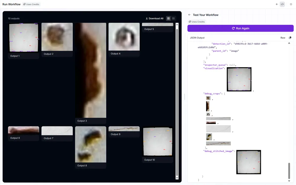
The merged output is called final_defects, containing all accepted and confirmed defects. Following is the output from workflow showing cropped and stitched images.
Step 4. Turn Detections into a Tile Verdict
Now that the confirmed defects are available, the workflow must decide whether to pass, reject, or inspect the tile. First, add a Detections Filter block called unresolved. It selects stitched detections whose classes are not hole, line, edge-chipping, or no_defect. This includes unsure and unrecognized labels. Next, add an Expression block named tile_verdict. Use the detection counts to apply these rules in order:
| Condition | Tile verdict |
|---|---|
At least one defect exists in final_defects | reject |
| An unresolved classification exists | inspect |
| The number of stitched boxes is smaller than the number of escalated boxes | inspect |
| None of the above conditions apply | pass |
The Expression block checks conditions in order and returns the first matching result. A defect in final_defects takes priority over an uncertain prediction. For example, if a tile has one accepted line defect and another detection marked unsure, the final verdict is reject. Human inspection is unnecessary because the tile already has a clear defect.
Step 5. Route Uncertain Tiles to the Inspector Queue
Tiles with the verdict inspect need human review. Add a Continue If block named inspector_gate with the condition tile_verdict == inspect. Only tiles that meet this condition continue to the review branch.
Use a Detections Combine block named review_labels to merge the accepted and escalated Stage 1 detections. The uncertain boxes retain their original Stage 1 classes so inspectors can review them. Next, connect the results to the Roboflow Dataset Upload block. Configure the block with the settings below.
target_projectas the tile defect project.persist_predictions = trueto save bounding boxes as pre-labels.registration_tags = ["cascade-inspect"]to identify review images.labeling_batch_prefix = tile_inspectwith daily batch creation.fire_and_forget = trueso the workflow can continue without waiting for upload completion.
The block also applies usage limits of 10 uploads per minute, 200 per hour, and 2,000 per day. Inspectors can open the uploaded images in Roboflow Annotate, review the existing bounding boxes, correct any mistakes, and approve the annotations. These reviewed images can later be added to the training dataset to improve Stage 1 through active learning.
Step 6. Add Escalation Metrics and Visualization
Monitoring helps determine how often Gemini is needed and whether Stage 1 is performing well. Add a Property Definition block named escalated_count. Use the SequenceLength operation to count the number of escalated bounding boxes for each tile. This value can be used to monitor escalation trends. If more detections start falling into the escalation band, Stage 1 may need better training data. For visual inspection, add two blocks:
- Bounding Box Visualization: Draws the final defect bounding boxes on the original tile image.
- Label Visualization: Displays each defect's class name and confidence score.
These blocks produce an annotated image that operators can use to check the detection results. The workflow also has a debug branch. Two more visualization blocks, debug_stitched_boxes and debug_stitched_labels, draw each stitched box with the class that Gemini gave it. The debug_stitched_image output returns that image. The debug_crops output returns the crops that Dynamic Crop sent to Gemini. Together, these outputs show what Gemini saw and how it labeled each uncertain box. The image below shows a test run in the Workflows editor. Output 1 is the final visualization. Outputs 2 to 9 are the eight crops that went to Gemini. Output 10 is the stitched debug image.
Step 7. Test Every Branch
Before deploying the workflow, test different tile conditions to make sure the escalation and verdict rules work correctly. The following table shows the expected results using mocked Stage 1 and Gemini responses.
| Stage 1 detection | Gemini response | Final verdict |
|---|---|---|
| line at 0.85 | Not called | reject |
| hole at 0.55 | hole | reject |
| line at 0.50 | no_defect | pass |
| edge-chipping at 0.45 | unsure | inspect |
| hole at 0.60 | Invalid class scratch | inspect |
| line at 0.42 | Unparseable response | inspect |
| hole at 0.30 | Not called | pass |
| No detections | Not called | pass |
| line at 0.85 and edge-chipping at 0.45 | unsure for edge-chipping | reject |
These cases check that high-confidence defects are accepted, uncertain detections reach Gemini, unresolved results go to the inspector, and confirmed defects take priority. The table represents expected results from local mocked tests. Test the same cases with real images and model responses before using the workflow on a production line.
Step 8. Run the Cascade from Python
After creating and deploying the workflow, use the Roboflow Inference SDK to process tile images from Python. The following script sends a tile image to the workflow and retrieves its results.
from inference_sdk import InferenceConfiguration, InferenceHTTPClient

client = InferenceHTTPClient(
    api_url="https://serverless.roboflow.com",
    api_key="YOUR_ROBOFLOW_API_KEY",
).configure(InferenceConfiguration(api_key_transport="header"))

result = client.run_workflow(
    workspace_name="your-workspace",
    workflow_id="tile-inspection-cascade-1791439720400",
    images={"image": "tile_0412.jpg"},
    parameters={
        "escalation_floor": 0.4,
        "accept_threshold": 0.7
    },
    excluded_fields=["visualization"],
)[0]

print("Verdict:", result["tile_verdict"])
print("Defects:", [
    box["class"]
    for box in result["final_defects"]["predictions"]
])
print("Boxes sent to Gemini:", result["escalated_count"])
The workflow returns three useful outputs:
tile_verdict: The final decision,pass,reject, orinspect.final_defects: The accepted and Gemini-confirmed defect detections.escalated_count: The number of detections sent to Gemini.
Running the script on one test tile prints the result below.

The tile is rejected because final_defects holds 18 defects. Eight boxes fell in the escalation band, so Gemini made eight calls for this tile.
The tile_verdict can be passed to a production controller through a PLC integration. For example, when the verdict is reject, the vision application can send inspection_result = FAIL to the PLC. The PLC then performs the configured rejection sequence.
Once deployed, monitor the escalation rate regularly to understand how often Stage 2 is needed and whether the cascade continues to reduce unnecessary inspections.
When a Cascade Isn't Worth It
A cascade adds moving parts. Two models, two thresholds, and a review queue all need care. Sometimes one model is the better choice. One rule covers many of these cases. Stick with a specialized detection model when "the output is bounding boxes, counts, or real-time tracking when no further interpretation is required." The table lists that case and five others.
| Situation | Why the cascade struggles | Better option |
|---|---|---|
| The output is only boxes or counts | A specialized detector already covers boxes, counts, and tracking. Gemini adds cost without new information. | Use a fine-tuned detector alone |
| Most boxes land in the band | Both stages run on most tiles. The p95 latency follows the Gemini path. | Improve Stage 1 with more data or a larger model before adding Stage 2 |
| Hard tiles are hard for Gemini too | Small defects that Stage 1 cannot judge are often hard for multimodal LLMs as well | Fix lighting, camera resolution, or training data |
| Rejects must happen at line speed | An escalated tile waits hundreds of milliseconds for a cloud call. The PLC write itself takes tens of milliseconds. | Run a larger local detector such as RF-DETR Large at 6.8 ms on a T4 |
| Tile photos cannot leave the plant | The Gemini block depends on a cloud API | Run a local VLM block such as the unified Qwen-VL block or Florence-2 on a self-hosted Inference server with a GPU. Another option is to escalate only to inspectors. |
| Tile volume is small | Two stages, thresholds, and monitoring cost more engineering time than the calls they save | Send every tile to Gemini and revisit the design as volume grows |
One test settles most cases. Run Stage 1 alone on a week of production tiles. Count the share of tiles with a box in the band. Then compare Gemini's answers with your inspectors' decisions on a sample of those tiles. A low escalation rate and high agreement mean the cascade will pay off.
If the numbers are not there yet, improve Stage 1 first. A better detector shrinks the band for every later stage.
Conclusion
A model cascade gives each tile the cheapest check that can settle it. RF-DETR handles the clear cases at line speed. Gemini reviews the uncertain boxes. Inspectors handle what is left. Each stage has its own threshold, latency, and cost. Each one can be measured and tuned on its own.
Start in Roboflow. Train a tile defect model. Build the workflow above. Then track the escalation rate on your own line.